Analysis of a simple Continuous Time Recurrent Neural Network (CTRNN) Model
Bits of brains
Introduction
Feedforward neural networks have neurons connecting from one layer to the next. In contrast, CTRNN is a neural network with connections forming a directed graph, which forms feedback connections. These feedback connections creates an internal state that exhibit dynamic temporal behaviour [8]. CTRNNs are used to model biological neural networks and frequently used in evolutionary robotics [2] [5]. Unlike with feedforward neural networks, which are reactive (i.e. classification or regression output to a given input), autonomous agents with dynamical neural networks such as CTRNNs can initiate action removed from current situation and organise behaviour with apparent future planning [1].
CTRNN neurons can be represented by the following ordinary differential equation

where
$y_i$ represents the state of the neuron $i$ and is updated by $dy_i$
$t_i$ is a time constant
$\theta_j$ is a bias term and
$I(t)$ is the external sensory input shared by all nodes.
$W_{ij}$ is the weight associated with the connection from $j^{th}$ neuron to the $i^{th}$ neuron
In this paper we would investigate the behaviour of it, starting with a simple neuron, using numerical methods and dynamical systems analysis, both analytical and graphi- cal.
Minimal neuron
We first start the analysis with a network containing a single neuron and constant input and no recurrent connection. Therefore the above equation (1) can be simplified to $$ \tau_i . \frac{dy_i}{dt} = −y_i + c \quad\quad(3) $$
where $W_{ij} = 0$ as $i = 1$, $N = 1$ & $j = 1$ (i.e. no recurrent connection) and $I(t) = c$
Behaviour of a dynamical system is primarily understood by analysing fixed points. Fixed points are the states that the system attracts to or repel from. In order to analyse the fixed points of this dynamical system, we set $\frac{dy_i}{dt} = 0$ Thus, there is a fixed point when $$ y_i = c \quad\quad(4) $$
Therefore fixed point is dependent on the external sensory input $c$.
We can plot the state of the neuron y by forward integrating through time using Euler method (5). Other more accurate methods exist, such as Runge-Kutta [6], but for simplicity we would use Euler. $$ y_{n+1} = y_n + hf(y_n) \quad\quad(5) $$
Where $h$ is a small value for e.g. $0.01$ and $f(y) = \frac{dy}{dt}$
Applying (3) results in
$$ y_{n+1} = \frac{ch}{\tau_i} +(1− \frac{h}{\tau_i})y_n \quad\quad (6) $$
Where $n$ is the time step. This equation essentially describes the system in discrete time.
In equation (6) Euler integration time step $h$ has a direct effect on the result. Analyti- cally, at the point where $h$ and $\tau_i$ are equal, $(1− \frac{h}{\tau_i}) = 0$ the stability of Euler integration is lost, and system behaviour can’t be captured. If $h$ is larger than $\tau_i$, integration does not capture the system behaviour, rather oscillates around it as shown in Figure 1. Therefore $h$ has to be smaller than $\tau_i$ for stable numerical integration.
We selected Euler integration time step to be $h = 0.01$ (and $\tau_i \geqslant1$) for subsequent experiments. Figure 2 Shows the change of state of the neuron when $c$,$\tau_i$ and $y_i$ changes and shows that the state of the neuron converges towards the external sensory input signal from its initial state. The speed of convergence is inversely proportional to $\tau_i$. The neuron's speed of response to an external sensory signal is therefore governed by $\tau_i$ which in a real neuron is composed of membrane resistance $R$ and capacitance $C$ such that $\tau = RC$ [3].
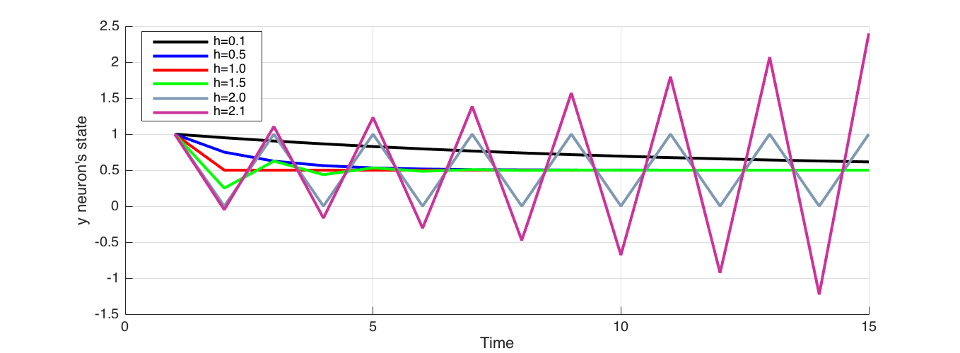
Figure 1 Effect of the choice of integration step $h$ compared to $\tau_i$. Here $\tau_i = 1$, Initial state of neuron set at 1 and the external sensory input at 0.5. When $h$ approaches $\tau_i = 1$, the integration results in coarser approximation and when they equal, jumps directly to the convergence without tracing the gradual decay. At $h=1.5$ integration oscillates about before eventually converging. At $h=2.0$ integration oscillates indefinitely, and when $h>2$ , integration oscillates about and diverges away.
Stability
Fixed points can be stable, meaning that small perturbations around it would lead the system state back to the fixed point. At unstable fixed points, small perturbations around it would lead the system state away from it, although if the system is already at that fixed point, it continues to stay there.
We analyse the stability of the fixed points identified above. Following on from equation (6), Let $F(y) = y_{n+1}$
$$ F(y) = \frac{ch}{\tau} + (1-\frac{h}{\tau})y \quad\quad (7) $$
Taking the derivative, $$ F`(y) = 1-\frac{h}{\tau} \quad\quad (8) $$
Fixed point as mentioned above equation (4) is at $y=c$
Stability of the fixed point are such that
$|F(c)| < 1$ when stable $|F(c)| > 1$ when unstable
$|F`(c)| = 1$ when semi-stable or periodic
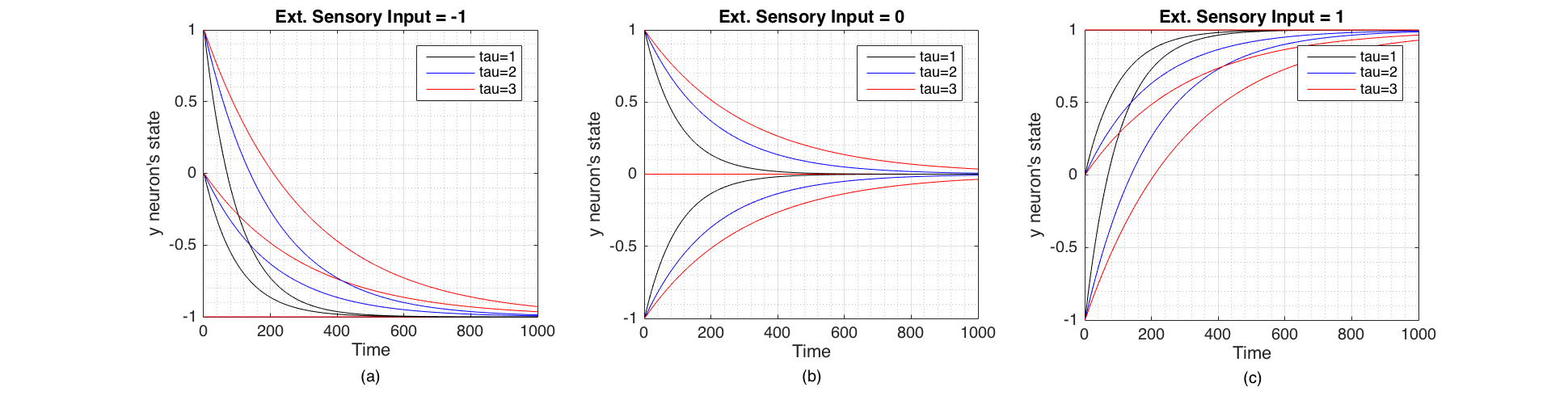
Figure 2 Change of state of the neuron through time plotted for three values of initial state $y_i$ (-1,0,1) and three values of $\tau_i$ (1,2,3). These were Euler integrated with $h=0.01$. (a) When the external sensory input is -1 (inhibitory). (b) When the external sensory input is 0 (no signal). (c) When the external sensory input is 1 (excitatory)
Since both $h$ and $\tau$ are greater than $0$, from equation (8) this means that, fixed point is stable when $h < 2\tau$, unstable when $h > 2\tau$, and semi-stable or periodic when $h = 2\tau$.
We can examine the latter case by substituting $h=2\tau$ in the equation (6), yielding the following for subsequent values of $y$ for the initial condition $y_0=k$

Therefore, when $h=2\tau$ the fixed point is periodic with period 2. Periodic fixed point would oscillate between two states as time progresses. This analysis can also be done using a graphical method called a 'cobweb plot' [7]
Re-forming equation (3) to the normal form, $$ \dot y = \frac{c}{\tau} - \frac{1}{\tau}y \quad\quad (9) $$ Shows that, this describes a first order linear system and therefore bifurcation does not exist. Bifurcation is a phenomenon where sudden appearance or disappearance of fixed points occur while changing a parameter. Bifurcation can be graphically analysed by plotting $\dot y$ against $y$ and then varying the parameter. As this equation (9) represents a line, there are no scenarios where a fixed point can be created or destroyed which results in qualitative change in behaviour.
Effects of varying external sensory input
We examine how the system defined by equation (6) behaves when the sensory input varies with time. First, we apply a sensory signal of 1 to the neuron for the first $n$ number of time steps and remove it subsequently.
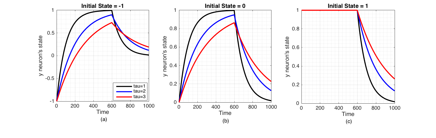
Figure 3 Change of state of the neuron when a excitatory sensory input ($I(t)=1$) is applied for the first 600 time steps only, plotted for three initial states $y_i$ (-1,0,1) and three values of $\tau_i$ (1,2,3). These were Euler integrated with $h=0.01$ (a) Inhibited neuron directly converges to the excitatory signal but decays to the ground state ($y_i=0$) when signal is removed. (b) Neuron in its ground state converges to the excitatory sensory input, but decays back to ground state when signal is removed. (c) Excited neuron stays at the same state when a excitatory sensory input is applied, but decays to ground state when signal is removed.
$\tau_i$ governs how quickly neuron responds to an external signal. Inhibitory external sensory signal ($I(t)=-1$) is similar to the Figure 3 but symmetrical over time axis. The above experiment simulates first pulse of a square wave. We can expect the neuron's state to change similarly for the rest of the pulses, if it was continued.
Figure 4 shows the response of the system to a periodic input (sine wave) which stops after 800 time steps.
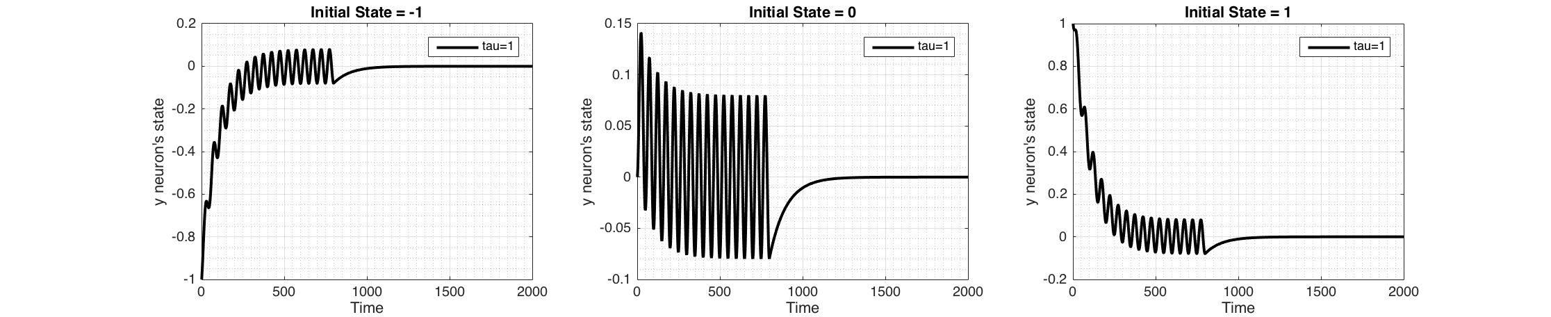
Figure 4 Change of state of the neuron when a periodic sensory input ($I(t)=sin(2\pi\frac{t}{50}$) is applied for the first 800 time steps only, plotted for three initial states $y_i$ (-1,0,1) keeping $\tau_i = 1$. These were Euler integrated with $h=0.01$ Sinusoidal signal has a dc-offset of zero, therefore the state of the neuron encodes the input signal and converges to the average of the periodic sensory signal which is zero. When the signal is removed, neuron converges back to its ground state.
Recurrent Connection
Now we consider a single neuronal system with a feedback connection to itself. Therefore the equation (1) becomes,

as $i=1,j=1,N=1$
and removing the subscripts for clarity as we are considering only one neuron here, $$ \tau \frac{dy}{dt} = -y + W\sigma(y+\theta) + I(t) \quad\quad (11) $$
This forms a one dimensional non-linear system, as $\sigma(x)$ is sigmoidal function, defined as equation (2). We investigate the behaviour of the system by forward integrating with Euler (equation (5)) we get, $$ y(t_{n+1}) = y(t_n) + \frac{h}{\tau}(-y(t_n) + W\sigma(y(t_n)+\theta) + I(t)) \quad\quad (12) $$
Figure (5) shows the behaviour of the recurrent neuron, in the absence of an external input for a range of values of $\theta$ and $W$.
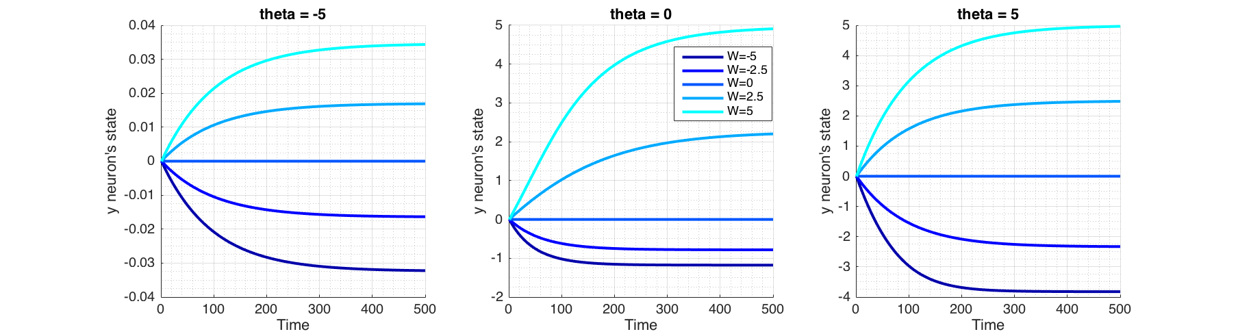
Figure 5 Behaviour of a recurrent neuron, in the absence of external input and initial state of $y=0$. Plotted for a range of values of $W$ and bias term theta ($\theta$).
In order for the fixed point analysis we would plot phase portrait ($\dot y$ against $y$) in Figure (6) as solving $\dot y = 0$ analytically is not possible. Fixed points and their asymmetry around time axis in Figure (5) are explained by the corresponding phase portrait plot in Figure (6), where fixed points are found at the intersection $\frac{dy}{dt}=0$, signifying that state doesn't change over time at these points. Arrows pointing towards a fixed point shows that at right side of the fixed point, $\frac{dy}{dt}<0$ thus reducing $y$, and on the left side $\frac{dy}{dt}>0$ thus increasing $y$, signifying a stable fixed point. Conversely arrows pointing outward from a fixed point signifies that it is unstable. In the case of a semi-stable, there would be one arrow pointing outwards.
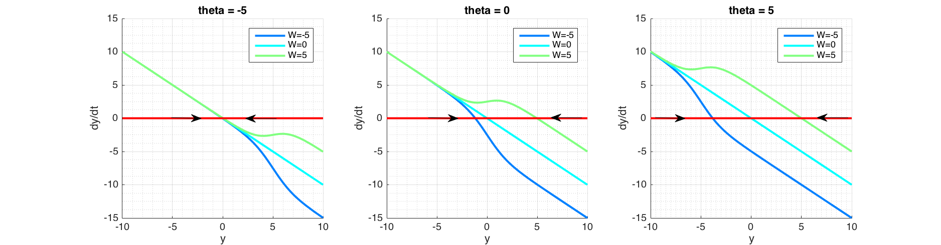
Figure 6 Phase portrait of a recurrent neuron, in the absence of external input and initial state of $y=0$. Plotted with a range of values of $W$ and bias term theta ($\theta$). For a given $W$, the bias term theta ($\theta$) determines fixed point location. For the given $W$ and $\theta$ values here, the fixed points are stable as shown by arrows converging. However bifurcation is possible with other values, see text.
For a given $y$, the bias term $\theta<0$, pushes the sigmoid away from activation (towards right; positive values of $y$) and when $\theta>0$, attracts the sigmoid to activation (toward left; negative values of $y$). This corresponds to plots shifting vertically as seen in Figure (6). Positive weight ($W$) reinforces the activation while negative weight inhibits it. $W=0$ equates to non-recurrent state.
Figure (6) shows that the system contains one fixed point for the values $\theta=[-5;0;5]$ and $W=[-5;0;5]$ and it is stable. But $W$ governs the curvature of the line and if for some value of $W>0$, this curvature forms a minima and a maxima that could cross $\dot y = 0$, creating a new fixed point, the behaviour would qualitatively change. We would examine this possible bifurcation scenario next.
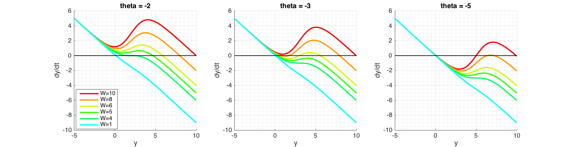
Figure 7 Phase portraits of possible bifurcation scenarios. At $\theta=-2$ (left plot) varying $W$ shows that at $W\approx4$, $F'(y) = 0$. Fixed point at this point is stable, but convergence would be much slower as $F(y)\approx0$. At $\theta=-5$ (right plot) increasing $W$ will create a second fixed point, which is unstable as $F(y)<0$ around it. Immediately after, a third fixed point will be created, which is stable as $F(y)<0$ on the right and $F(y)>0$ on the left. At $\theta=-3$ (middle plot) shows that increasing $W$ will make the middle fixed point to vanish by combining itself with the fixed point on the left.
Bifurcation
Bifurcation depends on $W$ and $\theta$ which are both independent. In order to examine the effects, we keep one parameter fixed while varying the other. Phase portraits shown in Figure (7) can be used to graphically reason out the stability of the system. Figure (8) shows 3 dimensional bifurcation plots as $W$ and $\theta$ are changed. Each point on the surface is a fixed point.
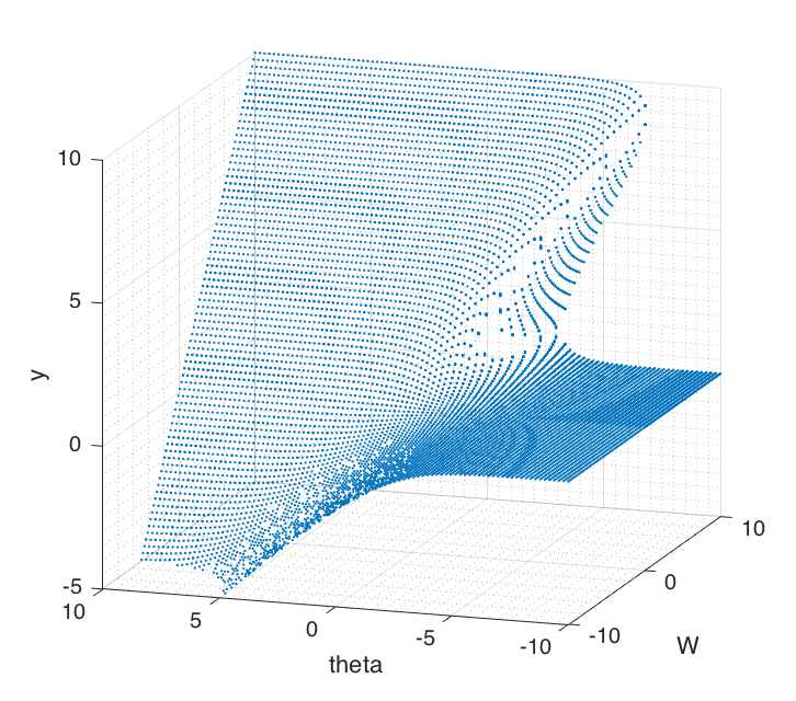
Figure 8 Bifurcation surface by plotting fixed points over ($W$ , $\theta$) plane. There's a 'cusp catastrophe' appearing when the surface folds over on itself.
It shows that the surface folds over on itself in certain places. This is called a 'cusp catastrophe' [4]. As parameters are changed, the behaviour of the system can discontinuously change, when there's a sudden drop over the surface above to the one below. In some real world systems like bridges, buildings or an insect ecosystem these could be truly catastrophic of its stability [4].
Finally with Figure (9) we try to understand what 'cusp catastrophe' means for this neuron, by changing the parameter $\theta$. When $\theta=7$ for all initial states, neuron returns to the ground state, which renders it a non-firing neuron. Conversely when $\theta=1$ for all initial states, neuron will activate, which renders it an always firing neuron. But at $\theta=-5$ firing of the neuron is dependent on its initial state.
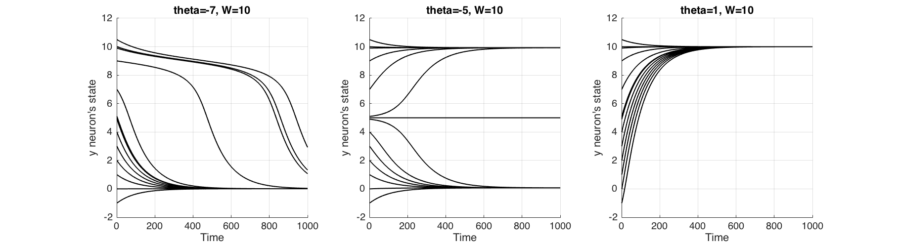 **Figure 9** The change of behaviour of the neuron when parameter $\\theta$ is changed. At $\\theta=7$ non-activating neuron, at $\\theta=5$ neuron activates depending on the initial state and at $\\theta=1$ neuron always activates.
Future investigations
As can be seen, a recurrent neural network with even a single feedback connection can have complex dynamics. Other avenues of investigation are available such as the behaviour analysis on an external input, and perhaps the dynamics of a two neuronal system.
References
[1] Randall D Beer. A dynamical systems perspective on agent-environment interaction. Artificial intelligence, 72(1):210–210, 1995.
[2] Randall D Beer. The dynamics of adaptive behavior: A research program. Robotics and Autonomous Systems, 20(2):257–289, 1997.
[3] Wilfrid Rall. Time constants and electrotonic length of membrane cylinders and neurons. Biophysical Journal, 9(12):1483–1508, 1969.
[4] Steven Strogatz, Mark Friedman, A John Mallinckrodt, Susan McKay, et al. Non- linear dynamics and chaos: With applications to physics, biology, chemistry, and engineering. Computers in Physics, 8(5):69–72, 1994.
[5] P.A. Vargas, E.A. Di Paolo, I. Harvey, and P. Husbands. The Horizons of Evolution- ary Robotics. MIT Press, 2014.
[6] Weisstein, Eric W. From MathWorld–A Wolfram Web Resource. Runge-kutta method., 2015. http://mathworld.wolfram.com/Runge-KuttaMethod.html.
[7] Weisstein, Eric W. From MathWorld–A Wolfram Web Resource. Web diagram, 2015. http://mathworld.wolfram.com/WebDiagram.html.
[8] Wikipedia. Recurrent neural network, 2015. https://en.wikipedia.org/wiki/ Recurrent_neural_network#Continuous-time_RNN.