On the effectiveness of Genetic Algorithms in training Feed Forward Neural Networks
Let's Evolve Neural Networks
Code for this experiment can be found on github
Introduction
Artificial Neural Networks (NN) are inspired by the biological neurons but are vastly simplified network of units with non-linear (or linear) activation, that can be used for many machine learning tasks belonging to broad categories such as classification, regression, data clustering or robotic control. It has been successfully applied in many fields from economics, financial, medical to marketing in recent times. There are many types of NNs, for example convolutional, or recurrent, here we consider the feed forward neural networks. This type of a neural network receives inputs on neuronal units on one end and the input is transformed and forward propagated through the network to produce an output on the other end.
Training a neural network for supervised learning (i.e. we tell the neural network what to learn) requires a labelled dataset and the aim is to learn a model from the data. This model would be represented by the weights of the connecting neurons and the topology of the network.
Neural networks predominantly rely on gradient techniques such as backpropagation (BP) for finding the minima in the error landscape. Here, the error landscape refers to the difference between the desired output as indicated by labels, and the actual output produced by the network with a given set of weights.
But these gradient techniques are inherently local and as such BP is sensitive to the initial conditions and learning rate, and on a complex error surface, it is very easy to converge to a local minima or get stuck in saddle points. Gradient diminishes to zero at a saddle point in the error landscape, but it doesn’t represent a minima. BP also requires the error function to be differentiable such that the gradient descent optimisation could work.
Genetic Algorithms on the other hand have very good characteristics in finding global optima efficiently on a complex landscape and differentiability is not a requisite and do not depend on the initial conditions. In previous studies, GAs had been applied in multidimensional problems such as aircraft design[6] and industrial controller design [5]. In 1999, Sexton & Gupta reported that GAs to be superior in training feed forward neural networks in chaotic time series approximation, in effectiveness, efficiency and ease of use [9]. In 2010, Zhen-Guo Che et. al. found that BP performs better but GA avoids over fitting [3].
In this set of experiments described, we applied BP and GA separately to 3 neural networks attempting 3 different tasks with increasing complexity to evaluate the performance of these two optimisation techniques, in terms of speed and effectiveness (level of reduction of error). We would show that despite these good characteristics, the GAs perform poorly compared to recent improvements to BP based neural network training techniques and are ineffective for modern deep neural network training.
Backpropagation
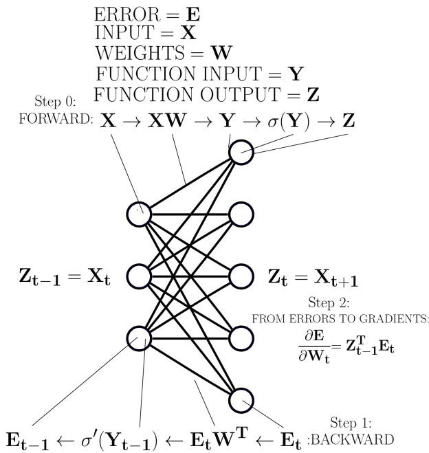
Figure 1 Backpropagation of an arbitrary layer in a neural network. Source: [7]
Backpropagation is the process by which the weights of a neural network is changed such that the error between the desired output and the actual output is reduced. The aim of neural network learning is to minimise this error summed over all training cases. The partial derivative $\frac{\partial E}{\partial y}$ (Where $E$ is the error and $y$ being the actual output of a layer) is numerically computed at each layer starting from the last, and in turn computing $\frac{\partial E}{\partial w}$ (Where $w$ represents the weight of a unit of a layer), the procedure is repeated for subsequent layers going back. The $\frac{\partial E}{\partial w}$ can be used to change the weights proportionally for each sample or accumulated over a batch. Gradient descent is then used as the optimiser in this n-dimensional weight-error space for error minimisation.[15].
This process can also be described as a set of rules [7], applied from the back of the neural network going forward as show in figure 1.
Multiply the error vector by the transpose of weight vector
Multiply the previous result element wise, with the derivative of the the activation function (i.e sigmoid) with respect to the inputs this function received from the forward pass
Repeat on the next layer going backward
Therefore, BP requires considerable amount of computing resources in terms of large matrix multiplications, and also large amount of memory to cache the results of the forward pass to be used by the backward pass.
History
Earliest deep learning networks can be traced back to Ivakhnenko and Lapa in 1965 [11]. These networks consisted of multiple layers which they trained with least squares fitting layer by layer. Backpropagation was available at this time, but it was inefficient and incomplete. It was derived in the modern form by Linnainmaa in 1970 [13] but was not presented as applicable to neural networks. As an important result in cognitive psychology in 1985 Rumelhart, Hinton and Williams showed that backpropagation in neural networks could yield distributed representation (connectionism) as features of a task [15]. In 1989, Yann Lecun was the first to use backpropagation in a practical implementation to create a convolutional neural network for digit classification. Recent resurgence of neural networks and deep learning where extremely large networks with billions of weights and hundreds of layers are trained with equally large datasets are a result of the abundance of computing resources such as GPUs, that can perform massively parallel large matrix operations.
Improvements
Many improvements have been made to NN learning techniques over the years: Stochastic Gradient Descent, ReLU, RMSProp, Dropout, L1/L2 Regularisation to name a few. Stochastic Gradient Descent (SGD) is a technique to speed up training time by using a random batch of samples for computing the average error, this is in contrast to using the whole dataset, which could take a very long time to perform gradient descent meaningfully. Rectified Linear Unit (ReLU) is a simplified non-linear activation function used instead of a logistic sigmoid. This speeds up training, by keeping the gradient from diminishing for large positive or negative values [14]. RMSProp is again a technique to make training faster, specially in the plateaus, when the gradient is extremely small, this ensures that the update take greater steps, so that gradient descent doesn’t get stuck in a saddle point. It also protects against exploding gradients, when encountered with a steep drop or a climb of the error space.
Over fitting is the phenomenon where the model fits to the training data without learning to generalise. This could happen when the dataset is small, not representative of the actual underlying model, when the training batch size is small, if the network contains more nodes than necessary. One method of avoiding overfitting is called regularisation. It modifies the loss function by adding terms to penalise large weights. Most common regularisation methods are called L1 and L2. Another method of avoiding overfitting is called Dropout [16], it prunes the network with some probability such that it learns to combine many possible topologies together to be efficient in using features.
We would come across these techniques in the experiments following, and show that these techniques make BP perform exceedingly better than what GA can offer.
Genetic Algorithms
Genetic Algorithms are a heuristic search and optimisation technique created by Holland J in 1975, loosely based on the process of natural selection and genetics. It consists of a population of search candidate solutions (individuals or a chromosome) consisting of units (a chromosome consisting of an array of genes) mapped to features of the optimisation task. The population is initialised randomly and then each individual is evaluated for its fitness by translating the genes into a set of features of the optimisation task. All individuals are evaluated and the ones with better fitness are allowed to continue to the next generation without modification, while the other half of the population get subjected to GA operators, mutation and crossover. This type of GAs called steady state, it lowers the computing memory requirement by not creating an extra offspring population, as usually the case for classic GAs.
Mutation is a process that creates a small random change in a gene of an individual’ chromosome at randomly selected loci. Crossover is a similar process that forces the less fit individual to accept parts of the chromosome from the fitter individual. There are many ways this crossover operation is done. Simplest is a single point crossover, where a crossover site is randomly selected and loser’s chromosome from there on, is replaced by the winner’s corresponding genes. Multi-point crossover is similar but with this process happening at a multiple set of loci. This type of one way crossover, is inspired by how microbes procreate, and adopted for its simplicity to lower the computing requirement.
Success of the GAs are due to the fact that they combine direction (by selecting the winners) and random chance (with mutation and crossover) in an effective manner and also, a population of these individuals contain more information about the search space than any one individual.
Experiments
We performed three experiments using two well known frameworks called Theano [1] [2] and Keras [4] that are accessible with Python programming language. For each experiment, we trained a neural network using backpropagation and suitable settings and recorded the speed of convergence as well as the loss decay. Then keeping the same network topology, we initialised weights and bias values, to represent the genes of a chromosome of the GA. Each gene in the chromosome, was a floating point value. We generated a population of chromosomes, each subjecting to GA operators, mutation and crossover, and computed the fitness by setting these values back into the corresponding weights and biases of the neural network and then evaluating the ’loss’ (mean squared error, mean absolute error, etc) in batches of the training dataset. The ’loss’ was used as the fitness value for each of the chromosome. Selection process was done by splitting the population into two groups and then comparing two to select the one with higher fitness (lower ’loss’). In order to keep the population diverse as possible, we subjected each layer’s weights and biases to mutation and crossover separately. The training was done using the training dataset and after training is finished (after a given number of epochs or generations). The loss was computed on the yet unseen testing dataset.
Single neuron regression task
We set up the network with a single neuron to perform a regression task, namely, to add two numbers together. We created a dataset of 600 floating point number pairs and their corresponding addition and also for testing, another 100 number pairs. These numbers were randomly generated and are between -50 and +50.
For BP based training we used a range of parameters (Table 1), best performing parameters were, mean squared error to compute the loss function and ’RMSProp’ as the optimiser with a linear activation and uniform initialisation of weights and the bias.
Loss function   Optimiser      Test Loss   Time (s)
--------------- ----------- ------------ ----------
MSE             AdaGrad          40.3155          1
MAE             RMSProp           0.0154          1
MSE             AdaDelta        0.001522          1
MSE             RMSProp       0.00008474          1
Table 1 Backpropagation based training on the single neuron regression task sorted by test loss. Test Loss, is the reduction of error reported on the test dataset. Lower test loss is better
For GA based training, we used single point crossover such that the loser of the tournament selection would get a portion of winners genes. We used a range of mutation and crossover probabilities as shown in Table 2. Best performing was mutation probability of 0.15 and a crossover probability of 0.5.
  pMutation   pCrossover   Test Loss   Time (s)
----------- ------------ ----------- ----------
        0.3       0.0001     1.01893         11
        0.3         0.25     0.07577         10
        0.5          0.5     0.04554         11
        0.3          0.5     0.02275         11
      0.075          0.5     0.02251         11
       0.15          0.5     0.01874         11
Table 2 GA based training on the single neuron regression task sorted by test loss. Test loss, is the reduction of error reported on the test dataset. Lower test loss is better
Backpropagation with RMSProp and mean squared error as parameters, performs orders of magnitude faster and converges to a much lower loss than the GA implementation.
AdaGrad optimiser uses an adaptive learning rate for each feature and more suited to finding discriminative features. In this case the features we are seeking are identical (i.e. weights both should ideally be 1), therefore its performance is lower.
Sine function fitting task
We set up a network with 3 layers with nodes 1-20-1 formation. We generated random set of numbers between -1 and +1 as the input dataset and the target dataset is the output of a sine function, added with some gaussian noise.
---------- ---------- ----------- -------- ------- --------- --------------
   Dataset Loss       Optimiser     Epochs   Batch      Test       Training
           function                           Size      Loss   time (mm:ss)
  1600/400 MAE        AdaGrad        50000      16   0.27104          24:16
     80/20 MAE        RMSProp        50000      16   0.29993          01:43
    160/40 MAE        RMSProp        50000       8   0.20800          05:24
  1600/400 MAE        RMSProp        50000      16   0.04991          29:58
  1600/400 MAE        RMSProp       100000      16   0.04155          59:23
---------- ---------- ----------- -------- ------- --------- --------------
Table 3 BP based training on the sine function fitting task sorted by test loss. Test loss, is the reduction of error reported on the test dataset. Lower test loss is better
BP based training with the parameters shown in Table 3 converges to a good solution in 30 minutes but a slightly better solution in an hour. The function fitting output shown in Figure 2 where the model generalises well ignoring the noise.
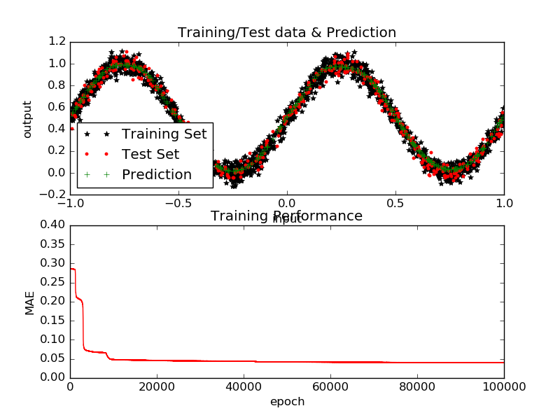
Figure 2 BP training and performance on the sine function fitting for minimum loss achieved (0.04155)
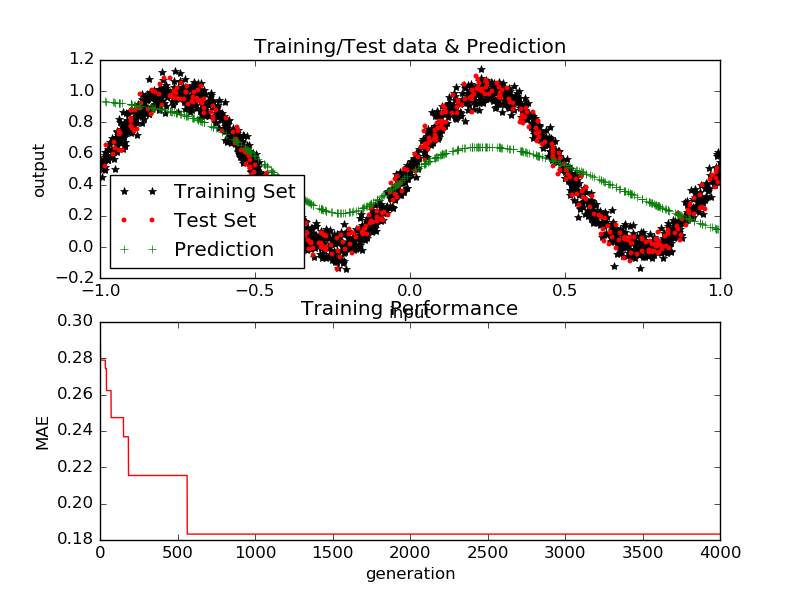
Figure 3 GA training and performance for Experiment w-09b with minimum test loss achieved 0.1359)
GA based training with various parameters is shown in Table 4. Best performing after comparable amount of time was experiment w-09b (Table 4). Initialisation contributed significantly for the better solutions, as well as the crossover, mutation rates and mutation factor. Figure 3 shows the function fitting output of the best solution found by the GA.
One of the main goals of the training is for the model to generalise well. We can see that with a larger dataset this generalisation becomes better (See Table 3). What this means is that, larger the dataset, the noise tends to average out and the features of the model have a better chance to be prominent. Therefore in reality having larger amount of data improves the model [10]. This generalisation is also affected by the size of the batch. With stochastic gradient techniques as used here, error is computed for a random batch of samples, as computing the error for the whole dataset takes quite a long while. With each batch, the error surface changes. So in essence the optimisation is done for an ever changing error landscape.
-----   ---------  ----------  --------  ------  -------  --------  -----------  -----  --------------
Test    pMutation  pCrossover  Training    Test     Time  Mutation  Generation/  Batch  Initialisation
                                 Loss    Loss  (mm:ss)    Factor   Population   Size
w-04         0.15        0.5     0.2366  0.2540    27:20       2.1     3750/200    533  zeros
w-08         0.85     0.0005     0.2389  0.2518    27:51       2.0     4000/200    533  rand(-1 +1)
w-03         0.15        0.5     0.1968  0.2040    28:50       2.0     1000/300   full  zeros
w-07b        0.15        0.5     0.1833  0.1823    27:51       2.0     4000/200    533  rand(-1 +1)
w-09a  0.15-0.187       0.75     0.1699  0.1680    33:57       2.0     4000/200    533  rand(-1 +1)
w-07a        0.15        0.5     0.1557  0.1563    27:11       2.0     4000/200    533  rand(-1 +1)
w-09b  0.15-0.183       0.75     0.1335  0.1359    29:53       2.0     4000/200    533  rand(-1 +1)
-----   ---------  ----------  --------  ------  -------  --------  -----------  -----  --------------
Table 4 GA based training on the sine function fitting task, sorted by Test Loss. Test loss, is the reduction of error reported on the test dataset. Lower test loss is better. Experiments w-09a and w-09b had a variable mutation rate which increased by 0.001 for 100 generations that best solution didn’t change. NN computes loss on a batch size of 16, and averages over number of batches available to it. The batch size reported here are the part of the dataset we used for training in a given generation. ’full’ means the whole dataset was presented and the NN would use a batch of 16 at a time and loss is averaged over the whole dataset. ’533’ means a random section of the dataset of size 533 was presented to NN at each generation, and NN uses a batch of 16 to compute the loss averaged over this section
With a small batch size, it’s easy to converge to a local minimum. Specially with GA, when it finds a solution with very good fitness early, most individuals in the population converges to this solution quickly, and lose the diversity within the population. But this solution may not be valid with newer samples defining the error surface differently. This may be addressed by increasing the mutation rate when the best fit doesn’t change for a number of generations. In our experiments increasing the mutation rate did not offer better solutions (Experiments w-05 & w-06 in Table 5).
------ ----------- ------------ ---------- -------- --------- ------- ------------ --
         pMutation   pCrossover   Training     Test      Time   Batch Generation
                                    Loss     Loss   (mm:ss)    Size Count
  w-05        0.15          0.5     0.1409   0.3069     00:19      16 750
  w-06    0.15-0.8          0.5     0.1973   0.2526     17:10      16 15000
------ ----------- ------------ ---------- -------- --------- ------- ------------ --
Table 5 GA based training effects of small batch size. The discrepancy between the training loss and the test loss indicates that model did not generalise well, even though, the training loss indicates that it is a good solution.
The behaviour of the steady state GA is such that, the winner gets promoted to the next generation unchanged. Therefore, in a changing error landscape this type of GA is unsuitable. Perhaps, a different method such as the one originally proposed by Holland J., where the next generation is made up by combining better performing individuals would be more suitable. This approach would allow a early false convergence to get diluted by later better solutions.
MNIST Handwritten character recognition task
In this experiment we attempt to recognise handwritten characters with well known MNIST dataset [12]. The Keras library contains this as an example, where the dataset is trained using a 512-512-10 network with 784 inputs consisting of flattened out 28x28 image into an array of numbers. We used 60,000 training samples and 10,000 testing samples.
-----------  --------  ---------  ------  -----  --------  ------  -------------
    Dataset  Loss      Optimiser  Epochs  Batch      Test    Test  Training time
 Train/Test  function                     Size   Accuracy    Loss  (mm:ss)
60000/10000  CCE             SGD      20    128    0.9572  0.1469  04:00
60000/10000  CCE         RMSProp      20    128    0.9849  0.0678  05:00
60000/10000  CCE         AdaGrad      20    128    0.9845  0.0565  05:02
-----------  --------  ---------  ------  -----  --------  ------  -------------
Table 6 BP Based training on MNIST data sorted by test loss. Loss function used is ’categorical crossentropy’ (CCE) which is more the default, and is more suited to image classification problems. Training performance over various optimisers listed, with all running for 20 epochs. As this is a classification task, we also have an accuracy measure (0-1 higher the better). Test loss is the loss reported on the test dataset.
----  ---------  ----------  --------  ------  -------  --------  -----------  -----  ----------------
      pMutation  pCrossover  Test        Test     Time  Mutation  Generations  Batch  Initialisation
                            Accuracy    Loss  (hh:mm)    Factor  /Population   Size
u-12       0.15        0.45  0.0969    2.2860  0:36          2.0      600/100    600  rand(-1 +1)
u-11       0.25        0.15  0.1911    2.2306  0:34       0.0001      600/100    600  rand(-0.0625 +0.0625)
u-05       0.15        0.50  0.3961    1.9399  1:23          2.0      2000/50    533  rand(-1 +1)
u-10       0.25        0.15  0.7072    1.5583  5:43      0.00001     3000/200    600  rand(-0.0625 +0.0625)
----  ---------  ----------  --------  ------  -------  --------  -----------  -----  ----------------
Table 7 GA based training on MNIST dataset sorted by the test loss. Test accuracy (0-1) is the classification accuracy on the test set.
Using BP for training with the default settings (RMSProp in table 6), 20 epochs complete in 5 minutes and yields a 0.0678 loss on test set with 0.9849 accuracy. Using GA for training we experimented with various settings for initial values, mutation and crossover probabilities and the mutation factor (i.e. the factor by which the floating point values of the genotype is changed). GA performed unfavourably compared to BP in all cases, even with extended training time as shown in Table 7.
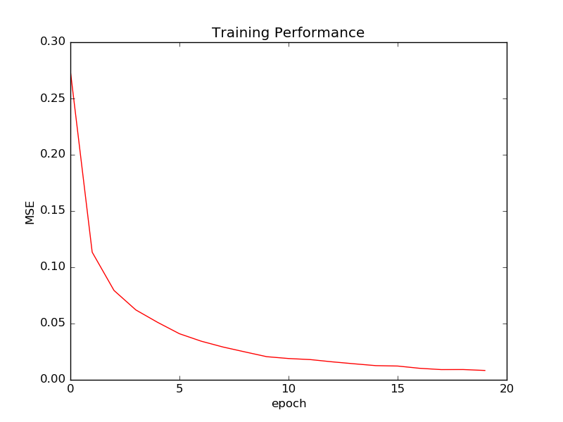
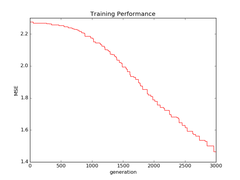
**Figure 4 ** MNIST dataset training loss decay. GA based training can continue for some more generations before the loss decay curve flattens out. BP based training is unlikely to improve much with more epochs.
MNIST character recognition task is a very small problem in the field of deep learning. The search space of the error landscape in this case is very large. For the GA to be successful, it is required to have a large population covering this space, so that there’s a better chance of an individual being in the vicinity of the optimum. But the computing resources are not enough to have a larger population in one computer. This would be a good candidate for parallelisation across machines in a network cluster. The superiority of BP comes through with the recent improvements and is quite capable of performing this type of a task very quickly, without requiring a huge cluster of machines or resources.
Conclusion
A lot of the problems with BP, has been alleviated, by various techniques described earlier in the backpropagation section. Problems like getting stuck in local minima is said to be happening less frequently in very high dimensional deep networks [8]. Saddle point are said be common, but with various techniques to combat those are available out of the box from modern neural network libraries like Keras, along with many ’hyperparamaters’ like this to be tuned depending on the problem.
GA lacks this type of varied tuning, apart from the usual parameters, mutation and crossover rates, population sizes and initialisation. These parameters don’t directly correlate with yielding a well performing neural network that could be trained in finite time. As shown from these three experiments GAs don’t scale well with the problem complexity. As the genotype gets large, the search space becomes exponentially larger requiring ever more larger population to effectively search the space. This is not practical, perhaps GAs would be more practical in tuning ’hyper-parameters’ of neural networks with backpropagation.
We performed three different tasks to evaluate the performance of a steady state GA compared to backpropagation in neural network training. In all three cases, BP was performing faster and yielded better results. The reported benefits of GA over BP in the previous studies have vastly been superseded by the recent improvements of gradient based training techniques.
References
[1] Bastien, Frédéric, et al."Theano: new features and speed improvements." arXiv preprint arXiv:1211.5590 (2012)
[2] JBergstra, James, et al. "Theano: A CPU and GPU math compiler in Python." Proc. 9th Python in Science Conf. 2010.
[3] Che, Zhen-Guo, Tzu-An Chiang, and Zhen-Hua Che. "Feed-forward neural networks training: A comparison between genetic algorithm and back-propagation learning algorithm." International Journal of Innovative Computing, Information and Control 7.10 (2011): 5839-5850.
[4] Franois Chollet. Keras - keras is a minimalist, highly modular neural networks library, written in python and capable of running on top of either tensorflow or theano., 2015.
[5] Chu, Baeksuk, et al. "GA-based fuzzy controller design for tunnel ventilation systems." Automation in Construction 17.2 (2008): 130-136.
[6] Chung, Hyoung-Seog, and Juan J. Alonso. "Multiobjective optimization using approximation model-based genetic algorithms." AIAA paper 4325 (2004).
[7] Tim Dettmers. [Deep learning in a nutshell: History and training, 2015.](http://devblogs.nvidia.com/parallelforall/ deep-learning-nutshell-history-training/)
[8] Goodfellow, Ian J., Oriol Vinyals, and Andrew M. Saxe. "Qualitatively characterizing neural network optimization problems." arXiv preprint arXiv:1412.6544 (2014).
[9] Gupta, Jatinder ND, and Randall S. Sexton. "Comparing backpropagation with a genetic algorithm for neural network training." Omega 27.6 (1999): 679-684.
[10] Halevy, Alon, Peter Norvig, and Fernando Pereira. "The unreasonable effectiveness of data." IEEE Intelligent Systems 24.2 (2009): 8-12.
[11] Ivakhnenko, Alekseĭ Grigorʹevich, and Valentin Grigorévich Lapa. Cybernetic predicting devices. CCM Information Corporation, 1965.
[12] Yann Lecun and Corinna Cortes. The MNIST database of handwritten digits.
[13] Linnainmaa, Seppo. "The representation of the cumulative rounding error of an algorithm as a Taylor expansion of the local rounding errors." Master's Thesis (in Finnish), Univ. Helsinki (1970): 6-7.
[14] Nair, Vinod, and Geoffrey E. Hinton. ["Rectified linear units improve restricted boltzmann machines." Proceedings of the 27th International Conference on Machine Learning (ICML-10). 2010.](Rectified linear units improve restricted boltzmann machines)
[15] Rumelhart, David E., Geoffrey E. Hinton, and Ronald J. Williams. "Learning representations by back-propagating errors." Cognitive modeling 5.3 (1988): 1.
[16] Srivastava, Nitish, et al. "Dropout: a simple way to prevent neural networks from overfitting." Journal of Machine Learning Research 15.1 (2014): 1929-1958.