Homeostatic Adaptation to Sensorimotor disruptions
Multilayered learning robots
Living beings are able to adapt to varying conditions in order to keep themselves alive. In normal conditions, they maintain their internal states by homeostatic adjustments. Can we device a simple agent to display these properties.
Code for this experiment can be found here
Introduction
Living beings are able to adapt to varying conditions in order to keep themselves alive. In normal conditions, they maintain their internal states by homeostatic adjustments. Regulation of body temperature is an example of homeostasis. Homeostasis consists of a mechanism to measure what's being regulated and a controller mechanism that can vary the regulated property and a negative feedback between these two mechanisms. In living beings, the ability to control body temperature allows them to live in a broad range of environments. The downside of this process is that it require higher expense of energy for the active control mechanism. The process of keeping itself alive with this type of adaptation is called ultra-stability.
Taking inspiration from this, Homeostat is an electromechanical device created by William Ross Ashby that demonstrates the adaptive ultra stability (Ashby, W. R. (1948, March 11)). It consisted of four conceptual parts as shown in Figure 1. In the ‘Ashby’s Mobile Homeostat’ paper (Battle, S. (2014)), which describes the homeostat in detail, authors note that - Ashby’s innovation was the double feedback loop augmenting the conventional sensorimotor loop, that models how the environment impinges on the organism’s essential variables. This is adaptation through ultra-stability.
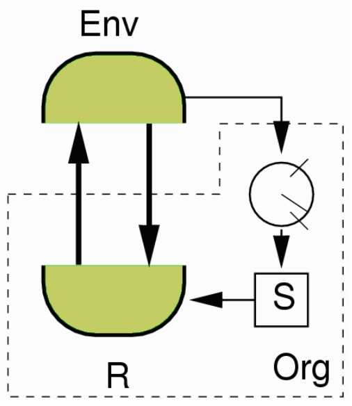
Figure 1. Ashby’s concept of an ultrastable system. Organism is represented by the unit enclosed in a dashed line. R is the behaviour generating subsystem which interacts with the environment represented by Env. Parameters that affect the actuators R, are represented by S. Circular meter represents the sensors which measure the effect on the environment with regard to the essential variables required for normal operation (keep alive). When the essential variables go out of bounds system becomes unstable and induces changes in S. It’s deemed to be adapted if the system can find an alternative equilibrium that maintains the essential variables with a new set of parameters in S. (Image source: Di Paolo, E. A. (2003))
This report discusses the replication of an experiment described in the paper titled 'Homeostatic adaptation to inversion of the visual field and other sensorimotor disruptions' (Di Paolo, E. A. (2000)). In this paper they study a virtual robot in the task of phototaxis as it had been evolved to perform, as well as, the homeostatic adaptation with sensory disruptions, which it had not been evolved for. The robotic controller is made up of a continuous time recurrent neural network and the intended behaviour is evolved using an evolutionary algorithm. Robots are evolved to perform long term phototaxis while maintaining homeostasis and then neuroplasticity is induced by a sensory disruption which forces the robots to adapt using methods of ultra-stability. This can be seen as an application of the Ashbyan ideas previously discussed, into evolutionary robotics.
This method uses plastic rules inspired by neuroscience, such as Hebbian learning (neurons that fire together, wire together) and BCM (Bienenstock,Cooper,Munro) theory of learning in visual cortex (Bienenstock et al., (1982)). BCM uses a sliding threshold for long term potentiation in which the threshold itself is governed by past synaptic activity.
Method
Physical Configuration
We created virtual robots whose bodies are represented by a circle with a radius 4 units Figure 2. They were able to move using the motors situated diametrically opposite sides of the circle. These motors enable them to move forward or backward. We modelled the speed of the motors to be directly governed by the controller and no momentum, acceleration, nor friction was modelled. This was to have a simple robot that can move toward a light source with the help of its controller. Motors can independently operate, directly connected to a governing neuron of the CTRNN (described below).
The light sensors were situated at the front of the robot with 60 (+/- 5) degrees from the body centre line on each side. These sensors were able to detect light which is modelled to be from a single source in the arena. There were no reflected lights or ambient light modelled. Light intensity was inversely proportional to the distance. Sensors had an aperture of 180 degrees and were forward facing. Occlusions were defined by the sensor embodiment.
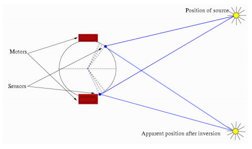
Figure 2. Robot’s physical architecture showing the location of sensors and the motors and how it would perceive the light source when the sensor connections are inverted.
CTRNN
The robots were controlled by an 8 node fully connected continuous time recurrent neural network (CTRNN). Sensors were connected to two nodes of the CTRNN, so were the motors albeit to different nodes. The parameters of the CTRNN (weights, biases, membrane potentials etc.) were evolved using a genetic algorithm along with other parameters we describe below. Neurons of the CTRNN is governed by the standard differential equation.

The $y_i$ represents the state of the neuron and zi represents the firing rate of the neuron. $w_{ij}$ are connection weights (range [-8,8]) from node $i$ to node $j$, and $I_i$ is the sensory input. Bias term $b_j$ had a range of [-3,3]. $\tau_i$ is a decay constant (range [0.4, 4]). All these parameters were evolved using a genetic algorithm.
Sensors and Motors
Light sensors and motors were applied with random noise with mean 0.25 and variance 0.25. Motors were driven by two selected neurons’ firing rates ($z_i$) remapped to the range [-1,1] and applied with a gain value in the range of [0.01,10]. The same gain range was applied to the sensory effectors as well. Gain values were also evolved. Sensor and Motor noise aids the discovery of the light source in the event of occlusions which unless stops the robot as momentum and acceleration were not modelled.
Plasticity Rules
There were 4 plastic rules (R0 to R4) associated with each connection weight, shown in Figure 3(a). Which rule would be assigned to a given connection weight was also evolved using a genetic algorithm.

Figure 3(a)
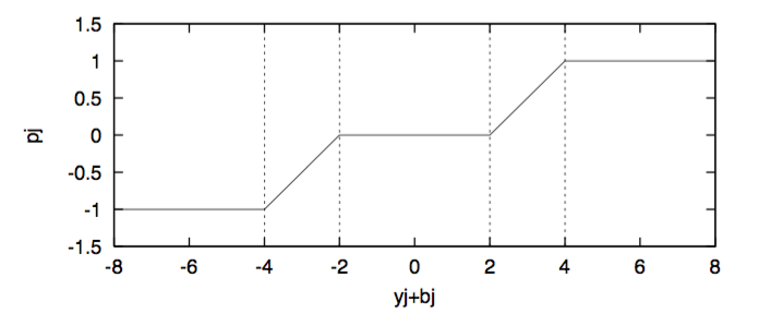
Figure 3(b)
$\eta_{ij}$ is a term that represents the strength and direction of the plastic change and has a range of [-0.9,0.9]. This parameter was evolved.
$\rho_j$ is the degree of local plastic facilitation which is dependant on $y_j+b_j$ and has piecewise linear relationship as described in Figure 3(b).
The $z^o_{ij}$ depends linearly on the weights such that it takes 0 when weight is at minimum and 1 when weight is at maximum.
The results of these equations are applied to the connection weights at each time step the CTRNN is evaluated. Rule 0 expresses the Hebbian/anti-Hebbian change associated with the pre and post neuron firing rate. Rules 1 and 2 affect the strength of the connection depending on the activities of pre and post neuron firing with respect to $z^o_{ij}$. These rules are local to a neuron and the plasticity applied doesn’t reflect the overall state of the robot.
Each neuron in the CTRNN was updated using Euler integration 5 times with the sensory input before motor output is set.
Genetic Algorithm
Each chromosome of the genetic algorithm is mapped to previously mentioned parameters and coded as a 148 floating point vector with values in the range of [0,1]. These values were mapped back to corresponding ranges of the parameters they represented. Gain values specified had an exponential scaling to its range, and in all other cases, scaling was linear. Mutation and crossover was set at global probability of 0.3 and uniform crossover was used. In addition to this floating point vector another integer vector of length 64 represented plasticity rules with values in the range [0,3]. Genetic algorithm was a steady state, microbial with elitism (Harvey, I. (2009)) and contained a population of 60 robots. The chromosome mapping is shown in Table 1.
| Weights | 64 | Motor Gain L | 1 |
| $\eta$ | 64 | Motor Gain R | 1 |
| Rules | 64 | Sensor Gain L | 1 |
| $\tau$ | 8 | Sensor Gain R | 1 |
| Biases | 8 |
Table 1 Genetic encoding map of the CTRNN parameters and sensor, motor gains, indicating how many elements are used for each. Rules are represented as integer vector where as the rest of the genome is encoded as a floating point vector.
Training
We created a population of robots and evolved them based on their ability to do phototaxis with homeostatic operation over 600 generations. For the 1st 100 generations the light source was at equal distance to all the robots, and in subsequent generations, the light source moves randomly by a distance in the range of [0, 500] at a random angle. At each generation we compute each robot's fitness using a combination of measures that promote non plasticity during normal firing of the neurons.
Fitness was computed with the following formula:
$Fitness = W_1 F_d + W_2F_p + W_3F_h$ $Fd = 1 - D_f / D_i$
Where $D_f$ = Final distance to source, $D_i$ = Initial distance to source, $F_p$ is the proportion of time a robot spends within 4 radii of the source for each generation. $F_h$ is the time average of the proportion of neurons that operated without plasticity (i.e. homeostatic). Weights, $W_1$, $W_2$, $W_3$ all add up to 1. $W_2$ had a range of $[0.64,68]$ and $W_3$ $[0.15,0.2]$.
In the original paper, the training was slightly more complicated where, the light source was moved multiple times during a generation. We simplified this process to not move during an evolving generation, but yet trained to seek the light source over a number of generations.
On the evolutions of the robots, we avoided the Lamarckian evolution by not setting the GA with the changed set of weights during the evaluation of the bots. This reduces the likelihood of evolving for specific task rather than for homeostatic adaptability.
####Simulation Environment Robot simulation environment is show below. The turquoise colours show that the bots are in plastic operation and the dark grey shows that they are in homeostatic operation. These states are updated for each simulation time step. Light source is shown in red while the flocking region is marked with red dotted circle. Robots paths can be seen drawn in light grey. Two graphs show the fitness (right) and the flocking ratio (left) for indication purposes.
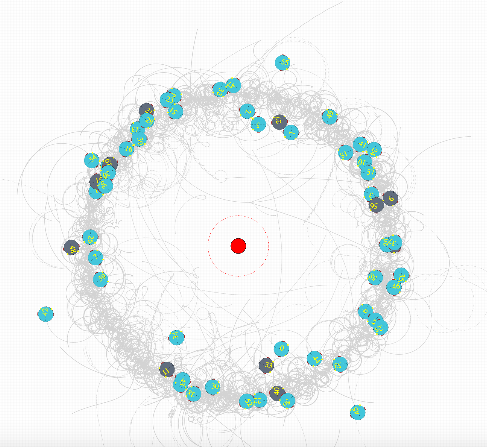
Figure 4(a). Initial stages of training. This shows that the at initial evolutionary stages most of the bots are not phototactic, and they mostly operate in plasticity.
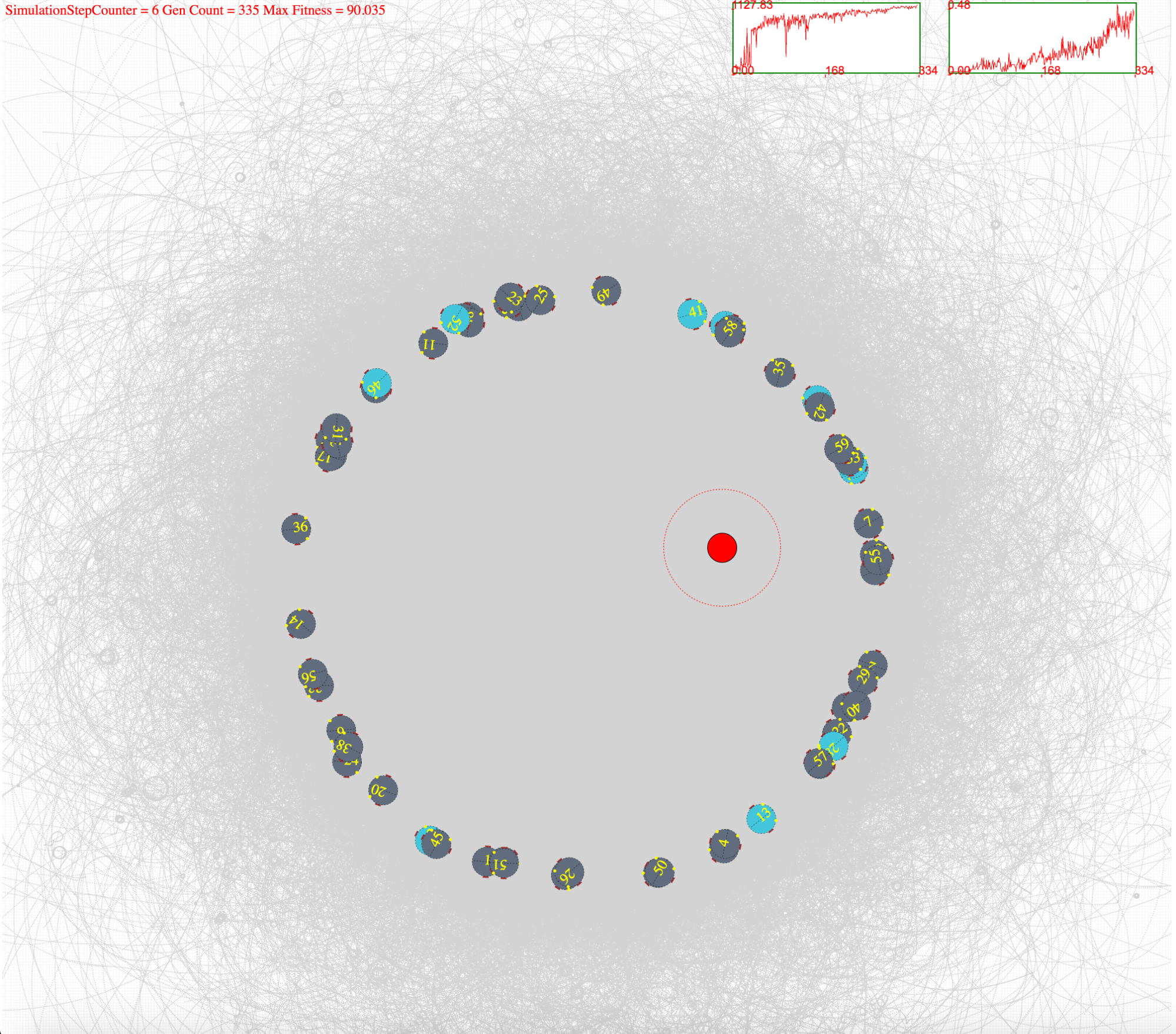
Figure 4(b). shows after few hundred generations of evolving, most of the bots operate in homeostasis. This depicts bots positions and states at the beginning of an epoch (500 simulation steps)
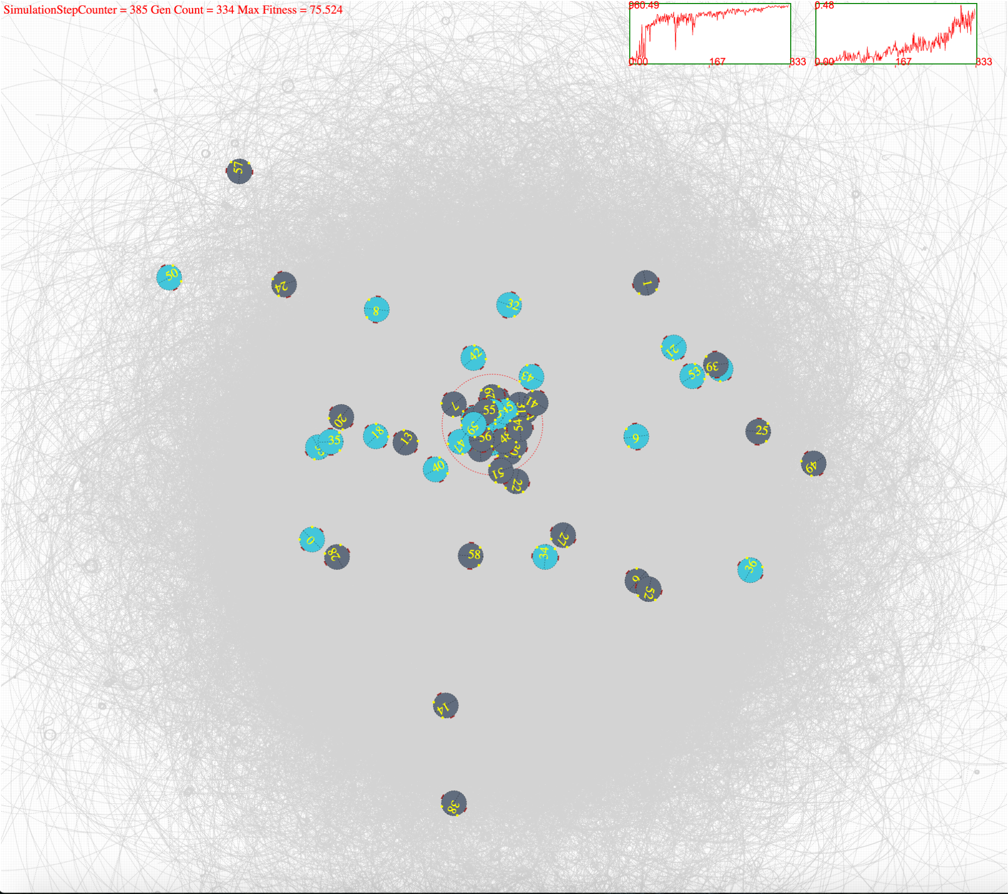
Figure 4(c). After few hundred generations of evolving robots are phototactic while being in homeostatic operation.
Results & Discussion
The results from the experiments widely varied between each trial. In most occasions if the bots were able to perform phototaxis, under normal sensory conditions, they were also able to perform phototaxis after sensory inversion. Upon inspection we discovered that, almost all the bots did not evolve to perform phototaxis with homeostasis rather they were using plastic rules all through out. With the plasticity intact, they were able to perform phototaxis after multiple sensor inversion cycles. Figure 5(a) and Figure 5(b) show this behaviour. Here the flocking is deemed to be performed if the bot stays within 4 radii of the light source at the end of the epoch. The figures presented are for the evolved best population (60 robots), averaged.
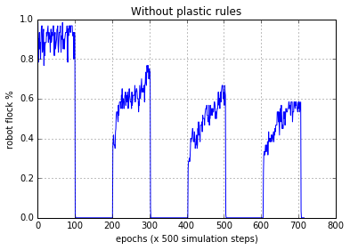
Figure 5(a). Robot behaviour without the plasticity rules operating. After 100 epochs the sensors are inverted, and after another 100 epochs the sensors are reverted back to normal. Each epoch consists of 500 simulation steps. As can be seen, when the sensors are inverted, the robots were unable to adapt to the sensory disruption and perform normal phototaxis.
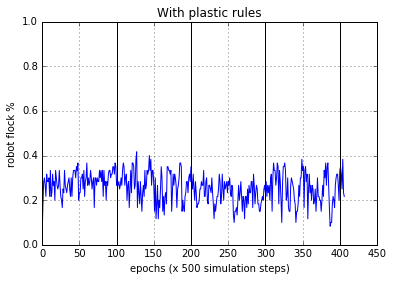
Figure 5(b). Robot behaviour with the plasticity rules operating. As can be seen the robots were able to adapt to the sensory disruption and perform normal phototaxis, when the sensors were inverted
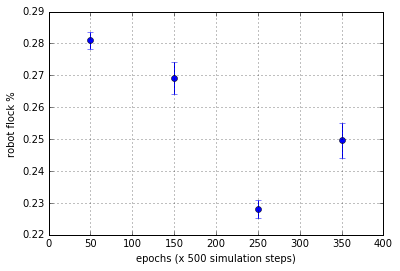
Figure 5(c). Flocking statistics for each 100 epoch segments c/f with Figure 5(b). Normal sensor orientation results in lower variance in flocking and Inverted sensors induce more variance. Mean flocking ability drops slightly in the first inversion (100-200 epoch range), but it is further degraded in the 2nd normal segment (200-300 epoch range).Sensor inversion and reversion has a long lasting effect on the robots on average.
In Figure 5(a), Robots start approaching the light source from equal distance. After each epoch, the light source was moved by a random polar coordinate which was 500 units from the current place. During the first 100 epochs robots were able to keep flocking to the light source in high numbers until the sensors were inverted at epoch 100. Light source was immediately available to them but flocking didn’t occur until the sensors were reverted back to normal at epoch 200. The flocking percentage gradually decreased at each inversion to normal transition, as the robots were moving further away in the arena while sensors were inverted.
During our experiments, with many evolutionary runs (~100) (each containing 600 epochs of training) only very few of the sets displayed the ability to phototaxis and homeostasis. This is mainly due to the way the fitness function was devised where the addition of Fp, Fd and Fh properties (described above in fitness function derivation) make up the fitness. Either phototaxis (Fp,Fd) OR homeostasis (Fh) can make up a winning individual, without having to have a combined association (which should be modelled by a multiplicative combination (AND) of these properties.)
This was addressed in the later paper titled 'Extended Homeostatic Adaptation: Improving the link between internal and behavioural stability' (Iizuka, H., & Di Paolo, E. A. (2008)) which discusses and offers possible improvements to the shortcomings of this method.
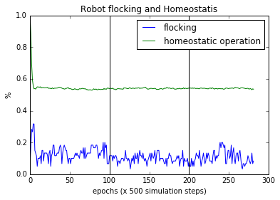
Figure 6(a). Flocking and Homeostasis. On average homeostatic operation of the bots remain constant after the initial drop even with sensory inversion. Sensory inversion happens at epoch 100 and revert to normal at epoch 200.
The association of homeostatic operation with the ability to adapt to sensory inversion can not be established even with the large number of trials we performed. As can be seen in the Figure 6(a), overall the homeostasis remains steady while the flocking continues when the sensory inversion occurs. This has been shown to be the case in the Extended Homeostatic Adaptation paper (Page 7, Fig 2 center) mentioned above .
In the following section we will look at the operation of individual bots to analyse their behaviour and homeostatic operations. Sensory inversion schedule is as before. Flocking is defined as bot remaining within 4 radii of the light source at the time of epoch finishing. As such this is a binary value, shown by 1.0 when flocked and 0.0 when not.
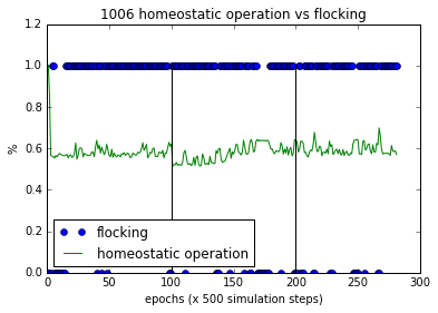
Figure 6(b). Flocking and homeostatic behaviour of a successful bot with homeostatic adaptation
In the normal operation segment (epoch 0-100) the homeostasis remains steady and at the inversion, it dropped indicating more plastic operations. Throughout the inverted segment, homeostasis increased while flocking continued, indicating that plastic rules influenced keeping the flocking to occur. The variance of homeostatic operations was higher than during normal operations indicating that plastic rules were acutely trying to keep the system operating as it was evolved to perform. This is an indication of ultra stability as described by Ashby.
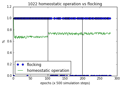
Figure 6(c). Flocking and homeostatic behaviour of a successful bot without homeostatic adaptation.
The homeostatic operation was quite steady during and after sensory inversion and reversal. With the sensory inversion, this bot increased its homeostatic operations. The number of flocking failures are increased after the sensory inversion,and its performance was affected long term by that. This demonstrates a mal-adapted bot albeit successful in phototaxis, as an example of the shortcoming of this method’s attempt to associate phototaxis with homeostatic adaptation.
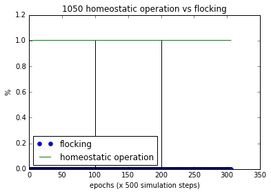
Figure 6(d). Flocking and homeostatic behaviour of an unsuccessful bot with homeostatic operation but without flocking ability.
This is an example of a robot that has only evolved to be homeostatic and not phototactic.
Extension
We experimented with a slightly different fitness computation function which aims to make homeostasis and phototaxis a unified goal. Following equation describes the fitness function used.
$Fitness = W_1F_d + 1000(W_2F_p * W_3F_h)$
Where $W_1 = 0.2, W_2 = 0.2, W_3 = 0.5$
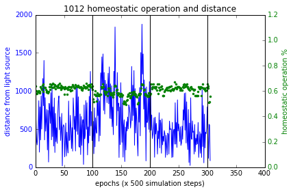
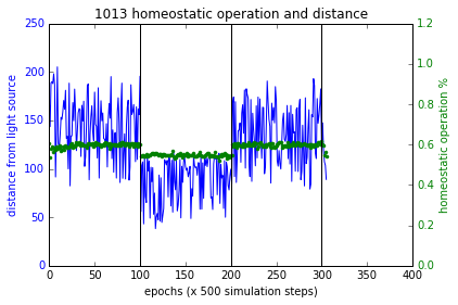
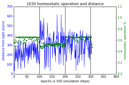
$F_p, F_d, F_h$ terms are as described above in section ‘Training’. $F_p$ and $F_h$ combined with multiplication as such in order for a higher fitness value, they both must increase together. Figure 4 (a,b,c) shows the simulations of these experiments and Figure 7 shows the results. Sensory inversion schedule is as before. With this fitness function more bots showing homeostatic adaptation were evolved compared to the method described in the paper. Although further analysis and improvements may be necessary, the initial results were promising.
 |
 |
|---|---|
 |
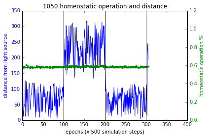 |
Figure 7 These plots show the performance of the new fitness computation, which yields bots that associate homeostatic operation with phototaxis at a higher likelihood. Plot at the bottom right shows a failure case where the bot had not used plasticity to regain phototaxis but it spends quite close to the source at the boundary of flocking (within 200 units from source). In all other cases, the bots became more plastic when the sensory inversion occurred (epoch range [100,200]) resulting in restoring phototaxis (or maintaining it) and when the sensors were reverted to normal, homeostatic operations increased.
Conclusions
Ultra stability observed in animals in abundance is an important goal for autonomous robotics (agents). This paper set out to devise a technique based on Ashbyan ultrastability hypothesis embodied in a minimal autonomous robot.
The method unfortunately doesn’t yield robots that can display ultrastability in a high degree of certainty. The method of fitness computation in evolving the agents play a considerable part in having only a tenuous association with phototactic behaviour and homeostatic operation. Therefore in future extensions as we have shown in our extension, the fitness computation must ensure that phototaxis and homeostasis are selected together in the evolutionary cycle.
As noted in the Extended homeostatic adaptation paper, the Hebbian-like rules tend to drive the connection weights to their extremes, resulting in loss of variability. Ultrastability depends on the ability to find new stable dynamics which benefits from having high variability in the connection weight landscape. In future extensions this should have a higher attention.
Looking at the biological counterparts, the homeostasis that maintains a biological regulatory system may have evolved first and then due to the environmental effects, evolutionary pressure may have arose to evolve a secondary regulatory system on top, leading to an ultra stable regime. This leads us to believe that homeostasis and the desired behaviour should be evolved first and once that is stable, the agents could be evolved further with various disruptions to the normal operations. This is in contrast to the emergent learning that the current method depended on. Interesting experiment would be to have a secondary CTRNN governing the plasticity in place of currently used rules.
References
Ashby, W. R. (1948, March 11). The W. Ross Ashby Digital Archive, Journals, vol.11, p2435. Retrieved from http://www.rossashby.info/journal/page/2435.html
Battle, S. (2014). Ashby’s mobile homeostat. In Artificial Life and Intelligent Agents (pp. 110-123). Springer International Publishing.
Bienenstock, E. L., Cooper, L. N., & Munro, P. W. (1982). Theory for the development of neuron selectivity: orientation specificity and binocular interaction in visual cortex. The Journal of Neuroscience, 2(1), 32-48.
Di Paolo, E. A. (2000). Homeostatic adaptation to inversion of the visual field and other sensorimotor disruptions.
Di Paolo, E. A. (2003). Organismically-inspired robotics: homeostatic adaptation and teleology beyond the closed sensorimotor loop. Dynamical systems approach to embodiment and sociality, Advanced Knowledge International, 19-42.
Iizuka, H., & Di Paolo, E. A. (2008). Extended homeostatic adaptation: Improving the link between internal and behavioural stability. In From Animals to Animats 10 (pp. 1-11). Springer Berlin Heidelberg.
Harvey, I. (2009). The microbial genetic algorithm. In Advances in artificial life. Darwin Meets von Neumann (pp. 126-133). Springer Berlin Heidelberg.