Simple Perceptron Classifier
Basic Binary Classifier
Perceptron looks as below:
              ------------------
X2 --- W2 -->|                  |   /-- +1 (if output > 0)
X1 --- W1 -->| Sum(Wi * Xi) + T |---
+1 --- T  -->|                  |   \-- -1  (otherwise)
              ------------------
This perceptron can process 2 features denoted by X1,X2 and has a bias which is set to +1.
The W1 and W2 are the weights associated with the features and T is the weight associated with the bias. Together they form the 'model' we would learn from the training dataset.
In this example, we generate the dataset such that,
XX1 represents the '+1' class
XX2 represents the '-1' class
Remember, each instance of the dataset contains 2 features and a bias. This is represented in a 3 element vector. Normally, the bias is a property of the neuron and doesn't change with the data. Here we attach it to the feature vector for the convenience of having the dot product do all the work.
We can create the train/validation split to be 80:20 such that XX1_train would contain 80 elements and XX1_val would contain 20 elements and similarly for XX2
Since we train the perceptron with traning data from both classes ('+1' and '-1'), we create a single training set called XX_train by concatenating XX1_train and XX2_train. (To be fair, we should shuffle the items so that we don't introduce a ordering based bias, but for this simple example we ignore that)
In Matlab, we can do the above steps as shown below
% We generate 80 data elements for the two classes with 2 features and a bias (set to 1)
c = 80
XX1_train  = [rand(1,c), 1 + rand(1,c), ones(1,c)];
XX2_train  = [rand(1,c), 0 + rand(1,c), ones(1,c)];

% Combine into one training set
XX_train = [XX1_train, XX2_train];

% We generate 80 corresponding labels for the above data elements
YY_train = [ones(1,c), -ones(1,c)];

% Similarly validation set can be generated as below
c = 20
XX1_val  = [rand(1,c), 1 + rand(1,c), ones(1,c)];
XX2_val  = [rand(1,c), 0 + rand(1,c), ones(1,c)];
XX_val = [XX1_val, XX2_val];
YY1_val = ones(1,c);
YY2_val = -ones(1,c)
YY_val = [YY1_val, YY2_val];
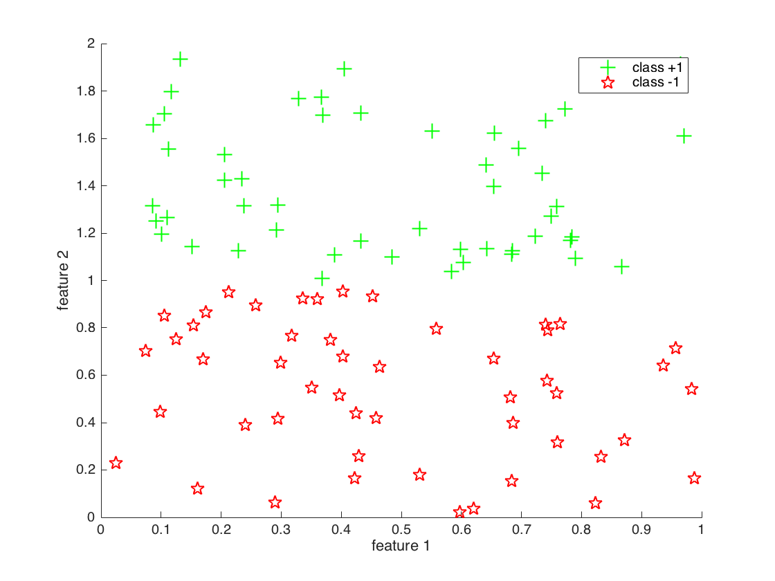
The generated dataset looks like this:

As can be seen, classes are linearly seperable because we made the 2nd feature vary between 1 and 2 by making (1+ rand(1,c)) in the code above.
Training
Now let's train the perceptron using the training set. The training algorithm looks like below:
For each data instance
    Predict the label
    Compare with the actual label
    if different, adjust weight by a small amount


Perform the above for a set number of iterations or
until some stopping criteria
(usually, until reduction of error falls below a threshold)
Matlab code would look something like this:
function [W] = TrainPerceptron(X,Y,K)
% X training dataset
% Y labels
% K number of training iterations

    W = [1,1,1] % initialise weights
    for j = 1:K % train K times
        for i = 1:M % iterate through all training data instances
            if sign(W' * X(:,i)) ~= Y(i) % evaluate the prediction
                W = W + X(:,i) * Y(i);	% adjust weights
            end
        end
    end
We can train the perceptron by calling the above function:
% Learn the model
model = TrainPerceptron(XX_train,Y_train);
#Predict Now that we have a model, it can be used for prediction using the validation set. The validation set is yet unseen by the model, so we can use it to evaluate how well our model predicts.
Here, we use the term 'validation set' loosely. Normally validation set is used for tuning hyper parameters and reduce over fitting.
Hyper parameters are various properties of a neural network like, number of layers, how many neurons are in each layer, etc.
Validation set is also used to reduce overfitting. This process is called Cross Validation. In machine learning, a good dataset is precious. It takes a considerable effort to create and assemble one, therefore it is in short supply. The aim of training a model is to use part of the data (training set) to learn relevant features of the underlying model and generalise well enough that it can be used for prediction on unseen data.
If we train the model too well on to the training set (overfitting), it is unlikely that it will perform well on unseen data. We combat that by splitting the 'would be training set' yet again into two - (Training and Validation). So we reduce the amount of training data, and carve out a portion that we can use for measuring how well the model performs. This type of partitioning is done multiple times in randomised fashion and performance measures are averaged.
So in summary, validation set is used to evaluate the model performance at training stage thus validating the model to be fairly trained.
Normally performance is evaluated and reported on a another dataset called the Test set. The test is used for final evaluation. There should be no more training rounds after testing set is used.
Data partitioning summary:
Total Dataset = [Training + Validation] + [Testing]
Cross Validation dataset partitioning:
[Training + Validation] = [TTTTTVV] | [VVTTTTT] | [TTVVTTT] | ...
With the following code, we can evaluate a few performance measures
TP = sum(sign(model' * XX1_val) == YY1_val); % True positives
TN = sum(sign(model' * XX2_val) == YY2_val); % True negatives
FP = sum(sign(model' * XX2_val) == YY1_val); % False positives
FN = sum(sign(model' * XX1_val) == YY2_val); % False negatives

accuracy = (TP + TN) /(TP + FP + FN + TN)
error = 1 - accuracy;
precision = TP / (TP + FP);
recall = TP / (TP + FN);
sensitivity = TP / (TP + FN);
specificity = TN / (TN + FP);
These measures aim to evaluate the model in different angles, as there isn't one measure that can paint the whole picture.
Precision = How relevant are the positive results. Recall (Sensitivity) = How good is the classifier detecting actual positives Specificity = How good is the classifier avoiding false alarms
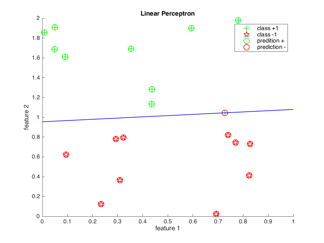
We can also draw the decision boundary. If we go back to the equation that gives us the output of perceptron given an input:
Y = W * X

% Where
% Y is the output
% W is the weight vector
% X is the feature vector (+ bias)
Now at the decision boundary, the output should be zero ( being neigther '+' class nor '-' class). Therefore, we can create a system of equations which looks as below:
[W1 W2 B] * [f1 f2 +1]' = 0

% Where
% W = [W1 W2 B]'  Weight vector
% X = [f1 f2 +1]  Feature vector
On a chart we draw f1 on x-axis, and if we select two points on the x-axis, we can compute the corresponding points on the y-axis with:
% W1 * f1 + W2 * f2 + 1 * B = 0
% f2 = (W1 * f1 + B) / -W2

% concretely
xcoord = [0.0 1.0];
ycoord = (model(1) * xcoord + model(3)) / -model(2)
And this is how it would look like for a different smaller dataset (as we are generating data)
